Uploads by Peter
From BoofCV
Jump to navigationJump to searchThis special page shows all uploaded files.
| Date | Name | Thumbnail | Size | Description | Versions |
|---|---|---|---|---|---|
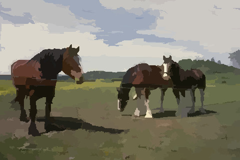
| 12:57, 10 June 2014 | Example Image Segmentation Color.jpg (file) |  |
30 KB | Segmented image where each region is assigned the average color of pixels inside. | 1 |
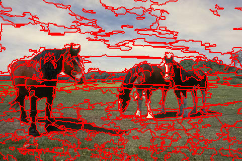
| 12:55, 10 June 2014 | Example Image segmentation Lines.jpg (file) |  |
89 KB | Segmented image where the borders are highlighted in red. | 1 |
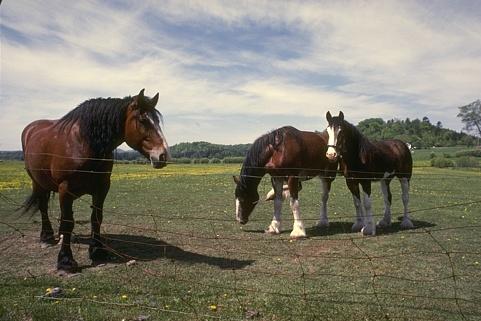
| 12:53, 10 June 2014 | Berkeley horses.jpg (file) |  |
30 KB | Horse image for segmentation from Berkley dataset: https://www.eecs.berkeley.edu/Research/Projects/CS/vision/bsds/ | 1 |
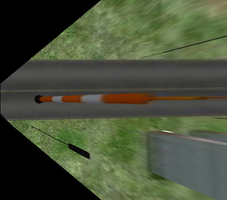
| 12:28, 10 June 2014 | Example dense optical flow.gif (file) |  |
166 KB | dense optical flow | 1 |
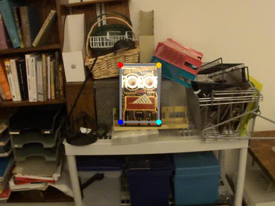
| 11:50, 26 December 2013 | Example tracking object.jpg (file) |  |
39 KB | Last frame from a sequence where the book was tracked using the circulant tracker. | 1 |
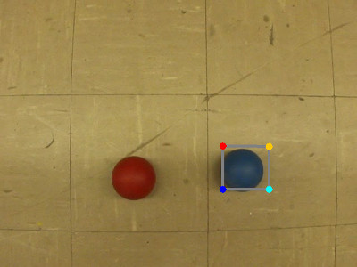
| 11:42, 26 December 2013 | Example tracking meanshift.jpg (file) |  |
24 KB | Last frame from a video sequence where mean-shift was used to track a color ball. | 1 |
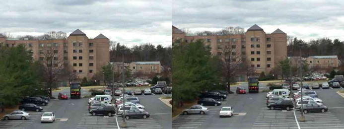
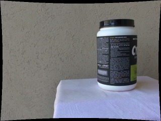
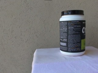
| 17:42, 25 December 2013 | Example video stabilization.jpg (file) |  |
58 KB | Input image on the left and stabilized image on the right. Hard to tell from a single image, but it has been stabilized. | 1 |
| 17:17, 25 December 2013 | Example remove perspective output.jpg (file) |  |
56 KB | Output image after a homography is used to remap the billboard and remove perspective distortion. | 1 |
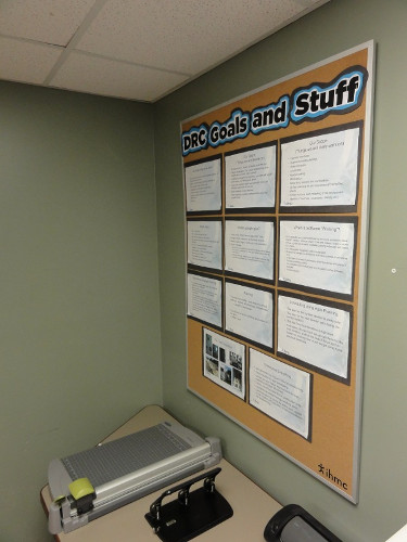
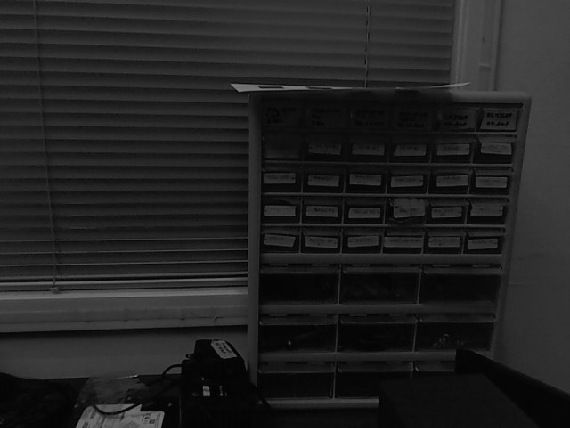
| 17:15, 25 December 2013 | Example remove perspective input.jpg (file) |  |
48 KB | Input file for removing perspective example. Note how the billboard is slanted. | 1 |
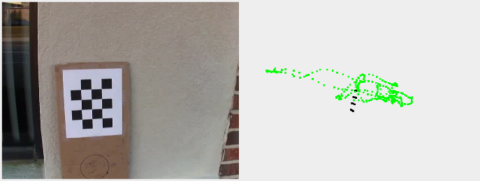
| 17:00, 25 December 2013 | Example calibration pose.jpg (file) |  |
31 KB | Image showing calibration target in the image and its trajectory from a side view. Green dots are the trajectory across the video sequence and black dots is the location of calibration points. | 1 |
| 16:44, 25 December 2013 | Example overhead output.jpg (file) |  |
35 KB | Synthetic overhead view created from input image and known ground plane. | 1 |
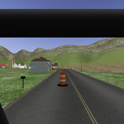
| 16:43, 25 December 2013 | Example overhead input.jpg (file) |  |
33 KB | Input image for computation of an overhead view. | 1 |
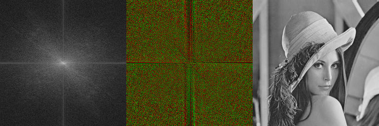
| 13:12, 25 December 2013 | Example dcf lena.jpg (file) |  |
67 KB | Visualization of the Discrete Fourier Transform as applied to the Lena image. | 1 |
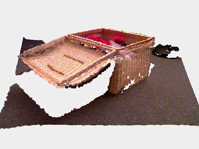
| 23:49, 19 June 2013 | Kinect point cloud basket.jpg (file) |  |
96 KB | Point cloud of an RGB and depth image from a kinect sensor. Synthetic view. | 1 |
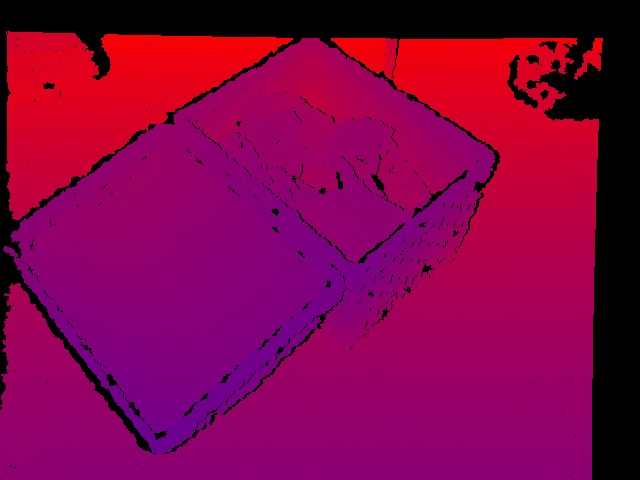
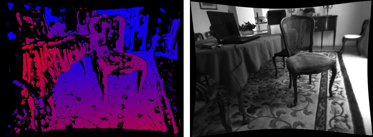
| 23:47, 19 June 2013 | Kinect depth basket.jpg (file) |  |
57 KB | Depth image from a kinect sensor of a basket. | 1 |
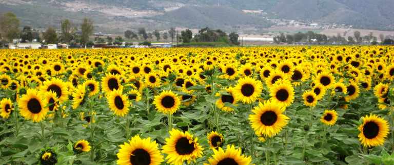
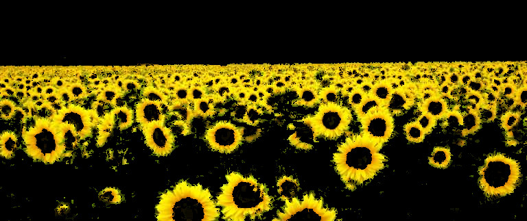
| 06:40, 15 April 2013 | Sunflowers.jpg (file) |  |
48 KB | Standard sunflow test image. | 1 |
| 06:32, 15 April 2013 | Example color segment yellow.jpg (file) |  |
119 KB | Image segmented using the color yellow. | 1 |
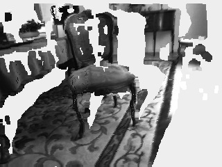
| 06:10, 15 April 2013 | Example stereo disparity3d pointcloud.jpg (file) |  |
29 KB | Point cloud used to generate a synthetic view of the scene. Created using a stereo camera. | 1 |
| 17:30, 14 April 2013 | Example image enhancement dark edge8.jpg (file) |  |
97 KB | Image with enhanced edges using 8 neighborhood algorithm. | 1 |
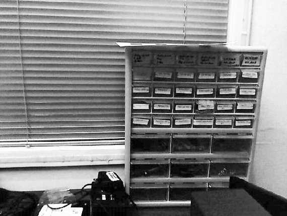
| 17:24, 14 April 2013 | Example image enhancement dark global.jpg (file) |  |
91 KB | Image after its global histogram has been adjusted for visibility. | 1 |
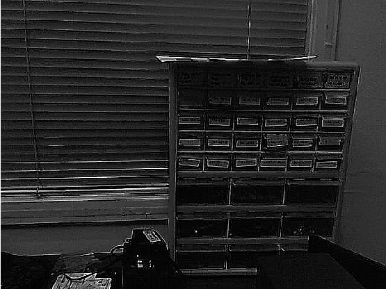
| 17:23, 14 April 2013 | Example image enhancement dark input.jpg (file) |  |
41 KB | Excessively dark image which is going to have its histogram adjusted. | 1 |
| 17:11, 14 April 2013 | Example fit polygon result.png (file) |  |
6 KB | The fitted polygons to inner and outter contours found from binary blobs. | 1 |
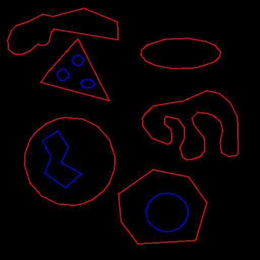
| 17:09, 14 April 2013 | Example fit polygon input.png (file) |  |
19 KB | Input image for polygon fit example | 1 |
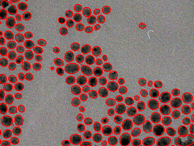
| 15:01, 14 April 2013 | Example fit ellipse.jpg (file) |  |
170 KB | Examples of ellipses fit to contours of binary blobs | 1 |
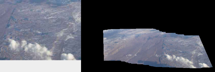
| 13:58, 14 April 2013 | Example video mosaic.jpg (file) |  |
44 KB | 2 | |
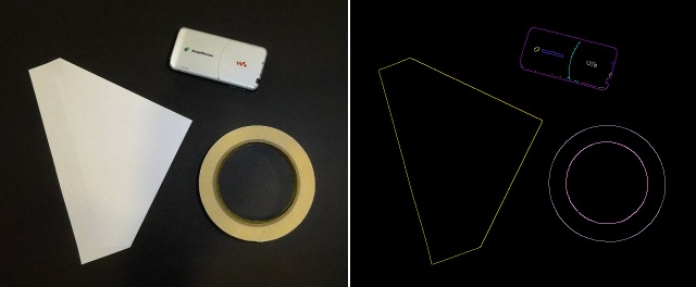
| 11:13, 14 April 2013 | Example binary contour.png (file) |  |
16 KB | Example of external and internal contours found in a binary image. | 1 |
| 17:25, 16 February 2013 | Example android video.jpg (file) |  |
40 KB | Demonstration of processing video on android by computing the image gradient and colorizing it. | 1 |
| 15:08, 16 February 2013 | Example uncalibrated rectification.jpg (file) |  |
93 KB | Better example image that is less pathological | 2 |
| 18:35, 5 December 2012 | Logo grace 125.png (file) |  |
30 KB | 2 | |
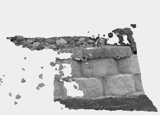
| 07:58, 18 September 2012 | Example mono stereo ptcloud.jpg (file) |  |
37 KB | 3D point cloud created from two views of a brick wall taken with a single camera. | 1 |
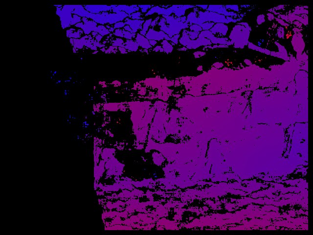
| 07:57, 18 September 2012 | Example mono stereo disparity.jpg (file) |  |
79 KB | Disparity image created from two views of a brick wall taken from a single camera. | 1 |
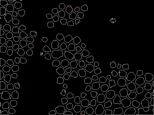
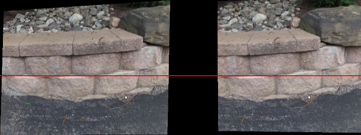
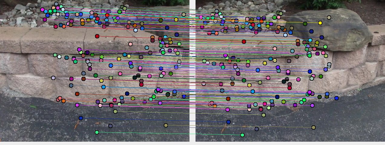
| 07:56, 18 September 2012 | Example mono stereo features.jpg (file) |  |
190 KB | Set of inlier features for essential matrix between two views from a single camera. | 1 |
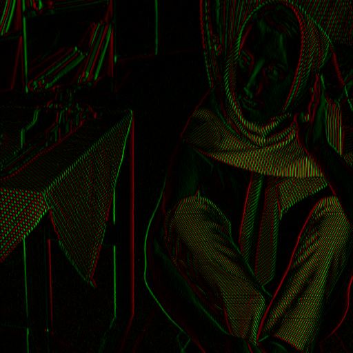
| 14:54, 22 July 2012 | Example convert visualize.jpg (file) |  |
41 KB | To visualize signed 16bit images it can be better to use one of the built in visualization functions which will colorize the pixel values. | 1 |
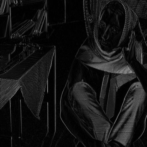
| 14:53, 22 July 2012 | Example convert scaled.jpg (file) |  |
52 KB | The 16bit edge image has had its absolute value taken and been rescaled so that it can fit into an 8bit unsigned image. | 1 |
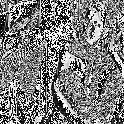
| 14:51, 22 July 2012 | Example convert bad.jpg (file) |  |
100 KB | Example of what happens when a 16bit image is converted into an 8bit image without rescaling its pixel values. | 1 |
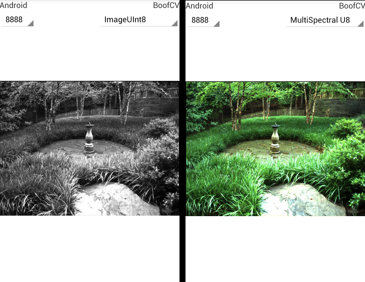
| 06:35, 18 July 2012 | Android benchmark app visual.png (file) |  |
395 KB | Android benchmark application visual verification. | 1 |
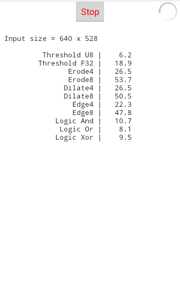
| 06:34, 18 July 2012 | Android benchmark app speed.png (file) |  |
28 KB | Android benchmark application's runtime benchmark in progress. | 1 |
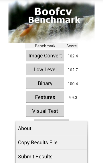
| 06:32, 18 July 2012 | Android benchmark app options.png (file) |  |
102 KB | Screenshot of Android benchmark application with the option's menu activated. | 1 |
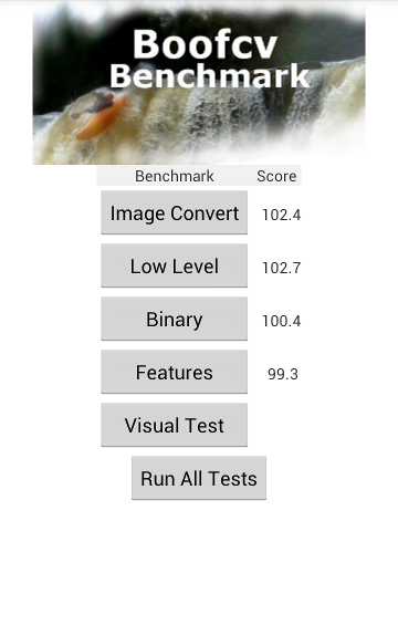
| 06:30, 18 July 2012 | Android benchmark app mainmenu.png (file) |  |
95 KB | Screenshot of Android benchmark application's main menu. | 1 |
| 15:24, 6 July 2012 | Object contours.jpg (file) |  |
30 KB | Original image and the found contour around the objects using a canny edge detector. | 1 |
| 20:53, 12 May 2012 | Example stereo disparity.jpg (file) |  |
191 KB | Disparity shown as a colored histogram from two calibrated rectified stereo images. Hot colors indicate a close object while cool indicates distant objects. | 1 |
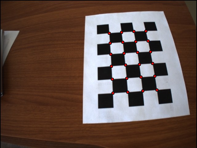
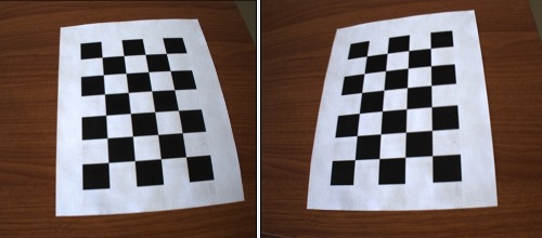
| 20:18, 12 May 2012 | Example chess calibration points.jpg (file) |  |
48 KB | Example of detected calibration points on a chessboard target | 1 |
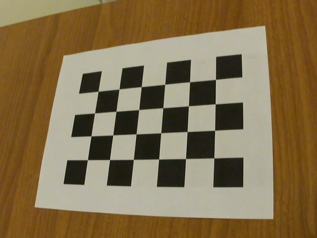
| 08:44, 12 May 2012 | ChessboardCalibrationPicture.jpg (file) |  |
36 KB | Calibration chessboard target example. | 1 |
| 15:59, 18 April 2012 | Example undistorted fullview.jpg (file) |  |
21 KB | Lens distortion has been removed from the image and adjusted so that the entire original image can be seen. The black regions are an artifact of removing lens distortion. | 1 |
| 15:57, 18 April 2012 | Example undistorted allinside.jpg (file) |  |
19 KB | Lens distortion has been removed from the image and it has been adjusted to maximize the view region without including pixels outside the original view. | 1 |
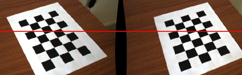
| 12:27, 18 April 2012 | Example unrectified.jpg (file) |  |
52 KB | Example of two stereo images before rectification. Note how the y-coordinate of feature do not line up. | 1 |
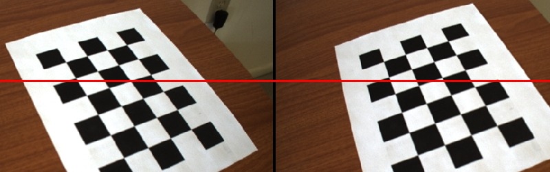
| 12:26, 18 April 2012 | Example rectified.jpg (file) |  |
49 KB | Example of a rectified pair of stereo images from a calibrated camera. Note how the y-coordinate of feature's line up? | 1 |
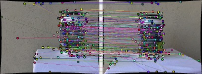
| 10:24, 18 April 2012 | Fundamental matches all.jpg (file) |  |
29 KB | Original set of feature matches before applying the epipolar constraint (Fundamental matrix). | 1 |
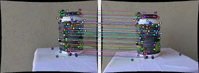
| 10:23, 18 April 2012 | Fundamental matches inliers.jpg (file) |  |
24 KB | Set of matched features after fundamental matrix has been computed using a robust algorithm. | 1 |
| 06:59, 18 April 2012 | Uncalib stereo.jpg (file) |  |
28 KB | Image of a calibration grid before lens distortion has been removed. Taken by a PtGrey Bumblebee camera. | 1 |