Tutorial Image Segmentation
Image Segmentation and Superpixels in BoofCV
This article provides an overview of image segmentation and superpixels in BoofCV. Image segmentation is a problem in which an image is partitioned into groups of related pixels. These pixel groups can then be used to identify objects and reduce the complexity of image processing. Superpixels are a more specific type of segmentation where the partitions are connected clusters.
The following topics will be covered:
- Thresholding
- Color histogram
- Superpixels
For a list of code examples see GitHub
Up to date as of BoofCV v0.17
Thresholding
- Global Thresholding
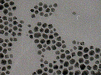
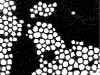
The most basic way to threshold a gray scale image is by thresholding. Thresholding works b by assigning 1 to all pixels below/above an intensity value to 1 and 0 to the rest. Typically the pixels which are assigned a value of 1 are an object of interest. BoofCV provides both global and adaptive (local) thresholding capabilities. The images above demonstrate a global threshold being used on a TEM image with particles.
Global thresholding is extremely fast, but it can be unclear what a good threshold is. BoofCV provides several methods for automatically computing global thresholds based on different theories. Otsu works by minimizing the spread of background and foreground pixels. Entropy maximizes the entropy between the foreground and background regions. The image's mean can also be quickly computed. The code below demonstrates how to compute and apply different global thresholds.
// mean
GThresholdImageOps.threshold(input, binary, ImageStatistics.mean(input), true);
// Otsu
GThresholdImageOps.threshold(input, binary, GThresholdImageOps.computeOtsu(input, 0, 256), true);
// Entropy
GThresholdImageOps.threshold(input, binary, GThresholdImageOps.computeEntropy(input, 0, 256), true);
The first two parameters is the input gray scale image and the output binary image. The 3rd parameter is the threshold. The last parameter is true if it should threshold down. If down is true then all pixels with a value less than or equal to the threshold are set to 1.
- Variable Lighting
A global threshold across the whole image breaks down if the lighting conditions vary within the image. This is demonstrated in the figure above. A calibration grid is the object of interest and spotlight affect can be seen. When a global Otsu threshold (center) is applied many of the squares are lost. Instead an adaptive threshold using a square region (right) is used and the squares are clearly visible. Adaptive thresholds based on squares and Gaussian distributions work well as long as there is sufficient texture inside the local region. If there is no texture then they produce noise. The figure below shows a text sample with a complex background being binarized. The adaptive square filter produces excessive noise, while the adaptive Sauvola produces a much cleaner image.
Below is a code sniplet showing how an adaptive square region (radius=28, bias=0, down=true) is applied to an input image.
// Adaptive using a square region
GThresholdImageOps.adaptiveSquare(input, binary, 28, 0, true, null, null);
// Adaptive using a square region with Gaussian weighting
GThresholdImageOps.adaptiveGaussian(input, binary, 42, 0, true, null, null);
// Adaptive Sauvola
GThresholdImageOps.adaptiveSauvola(input, binary, 5, 0.30f, true);
See JavaDoc for a complete description of each of these functions. null values indicate an optional input image for internal work space. Supplying the work space can reduce overhead by creating/destroying memory. When using Sauvola it can be faster to create ThresholdSauvola directory and reuse the class for each image which is threshold. Sauvola requires several internal images for storage and creating all that memory can become expensive.
- Difficult Text Example
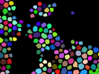
After an image has been thresholded how do you extract objects from it? This can be done by finding the contour around each binary blob. In the code sniplet below the outer and inner contours for each blob is found. In the output "label" image pixels which belong to the same blob are given a unique ID number. The contour of blobs is critical to shape analysis. A visualization of the labeled blobs is shown below.
List<Contour> contours = BinaryImageOps.contour(filtered, ConnectRule.EIGHT, label);
- Blob Extraction
Examples
Thresholding API
Color Histogram
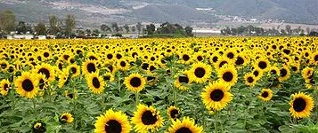
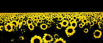
Next up is color based image segmentation. Color based segmentation assigns pixels to a region based color information alone. In the above example all the pixels which are approximately yellow are saved and the rest are set to black.
BoofCV does not provide a highlevel interface for color based segmentation, but does provide the tools you will need implement it yourself. The color space in which segmentation is performed is important. The most common color space, RGB, is not invariant to changes in lighting, while HSV is. This can allow for a simpler function to be used. Example code is provided (see below) which does exactly this. When the example code is run, you can click on the image and it will segment out all pixels which have a similar appearance.
In the video below, color segmentation was used to identify the road in a simulated environment and steer the car.
Examples
Superpixels
Superpixels are sets of connected pixels which have similar features. The border region between superpixels tends to lie along the edges of shapes. Different algorithms will produce superpixels of different shapes, see figure above. For example, SLIC produces regions which are approximately the same size while Felzenzwalb-Huttenlocker (FH) and Mean-Shift produce a variable number of regions depent on the scene's complexity.
One of the earlier superpixel algorithms is watershed. The idea behind watershed is that the image is viewed as a topological map where pixel intensity is the pixel's height. If you placed a waterdroplet in any of pixels it would fall down towards a local minimum. All pixels which fall inside the same local minimum belong to the same superpixel. While very fast, it tends to over segment images.
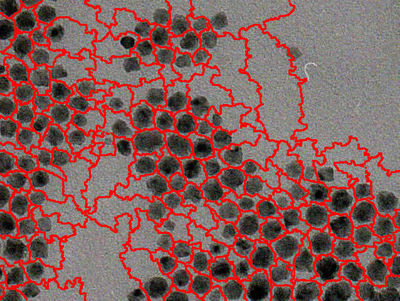
To overcome watershed's oversegmentation issue you can provide a seed to initialize each region. How you generate the seed is dependent on the application. In the image below seeds were found using a blob detector. If seeds were not used then there would be thousands more regions due to the amount of noise in the image.
A code example is shown below demonstrating superpixel segmentation using the ImageSuperpixels highlevel interface. FactoryImageSegmentation should be used to create new instances of ImageSuperpixels.
	ImageSuperpixels alg = FactoryImageSegmentation.fh04(new ConfigFh04(100,30), imageType);
	GrayS32 pixelToSegment = new GrayS32(color.width,color.height);
	alg.segment(color,pixelToSegment);
Superpixel Summary Table
| Name | Count | Color | FPS |
|---|---|---|---|
| Mean-Shift | Variable | Color | 0.5 |
| Gray | 0.8 | ||
| SLIC | Fixed | Color | 1.8 |
| Gray | 2.4 | ||
| Felzenszwalb-Huttenlocher | Variable | Color | 5.1 |
| Gray | 5.2 | ||
| Watershed | Both | Gray | 43 |
FPS (Frames Per Second)was found using a 481x321 image on a Intel Core i7-2600 3.4 Ghz, single thread. Count is the number of regions it will find in an image. Color indicates if a color or gray image was processed.
